In Excel, there are many instances when you may need to compare two columns. It is simple when there are only a few columns and rows, but as the table expands, you need to scroll horizontally or hide columns to create a comparison.
Often, it might require you to manually compare and write down as ‘Match’ or ‘Not Match’ or highlight the matching or mismatching data in each column.
Manual comparison is painstaking and might lead to erroneous data. However, there are many methods to streamline this process.
Why Is It Useful to Compare Two Columns in Excel?
Excel spreadsheets are useful for data storage, manipulation, and decision-making. It's not good at crunching numbers but it is a versatile tool for formatting text.
Features such as comparing two columns help data analysts to make informed decisions based on data. Mainly, a data analyst compares two columns across the same or different spreadsheets. Manually comparing columns is a tedious task, and it involves hours or probably days if data goes missing.
Comparing two columns in Excel is highly imperative for a data analyst to determine whether the cell contains data. Excel displays it as TRUE/FALSE, Match/Not Match, or other user-defined messages.
How Do You Compare Two Columns in Excel?
When you have data in two columns, tables, or spreadsheets, you may often need to compare them to see what data is missing or present in both. Comparisons can happen in many different ways for different reasons.
Depending on what you want, specific methods need to be used to compare columns. You can compare two columns in Excel by:
- Highlighting the unique or duplicate values in each column using functions.
- Displaying unique or duplicate cells using conditional formatting or formulas.
- A row-by-row comparison.
- Using LOOKUP formulas.
Comparing Two Columns in Excel with the Equals Operator
You can compare two columns, row by row, and find the matching data by returning the result as Match or Not Match. The formula used is =column1=column2, and by default, Excel returns a True if there's a match or else False.
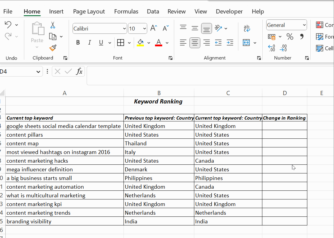
In cell D4, insert the formula =B4=C4 and press Enter. Then, drag it down to the end of the table. The formula returns TRUE if the values in compared columns are the same or returns FALSE if the values differ.
Compare Two Columns in Excel Using the IF Condition
You can compare two columns using the IF condition in Excel. The formula to compare two columns is =IF(B4=C4,”Yes”,” ”). It returns the result as Yes against the rows that contain matching values, and the remaining rows are left empty.
The same formula can identify and return the mismatching values. You need to include an additional argument, No, when the IF condition proves false. The formula is =IF(B4=C4,”Yes”,”No”).
To compare two columns in Excel for differences, replace the equals sign with the non-equality sign (<>). The formula is =IF(A2<>B2,”Match”,”Not a Match ”).
Compare Two Columns in Excel Using the EXACT() function.
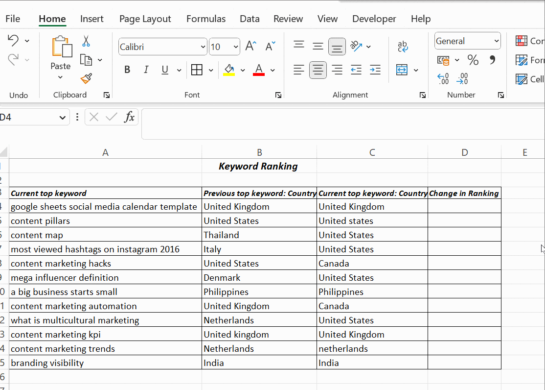
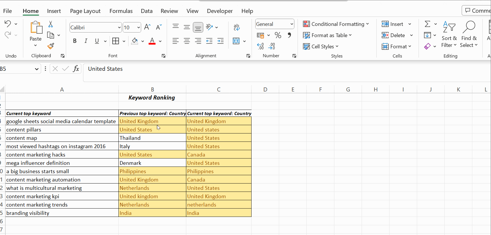
If you noticed in the previous screenshot, the formula returned a Yes for matching results that had different capitalizations.
For instance, the country names had different capitalizations in rows 5, 13, and 14. The IF() returned Yes while comparing two columns containing Netherlands and netherlands, with n in lower case.
If you wish the capitalizations to be identical, use EXACT() when comparing two Excel columns and IF().
The EXACT() function compares two text strings and returns Yes only if they have the same capitalizations.
EXACT is case-sensitive but ignores formatting differences. The syntax is =EXACT(text1,text2). It takes two arguments, text1 and text2; both are required when using this function.
Let’s look at some examples. This time, EXACT() is used along with IF().
Use the formula =IF(EXACT(B4,C4), "Match", "Mismatched") for the IF condition to be case sensitive.
As you can observe, it returns the result as Mismatched for columns with matching results yet mismatched capitalizations.
The execution of the formula is as follows: first, the inner function is executed, and the result is returned. In the above example, the EXACT() function returns a false value to the outer function IF.
The general working of the IF condition is that if it returns true, the first argument in the function is returned. Or the second argument is returned as false.
Compare Two Columns in Excel Using Conditional Formatting.
Click Home, then on Styles.
Then, follow these steps Conditional Formatting → Highlight Cell Rules → Duplicate Values.
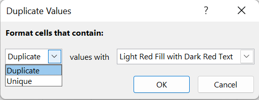
You get a dialogue box, as shown below. From there, you must choose the values from the drop-down menu.
Apply the formatting condition on the cells. You can choose any conditions; Duplicate or Unique.
Format cells that contain: (options) values with (options).
Use Conditional Formatting to find and highlight the data that are present in both columns. Before using conditional formatting, select the columns required for comparison.
Choose Duplicate if you wish to find the names in both columns. To highlight it, choose any options: filling with colour, changing the text colour, or changing the cell border.
The last option is a Custom Format. Choose this option if you wish to highlight the cell with a colour of your choice other than the ones specified in the drop-down menu.
Another option that you can use is ‘Unique.’ Use this option if you are interested in highlighting the cells that contain data that is not repeated. That is, you wish to highlight the unique cells.
Instead of selecting Duplicate, choose Unique from the drop-down list, and apply any options, such as filling with colour, changing the text colour, or changing the cell border.
Tip: If you wish to clear the formatting you performed on the cells, click Conditional Formatting → Clear Rules → Clear Rules from Selected Cells.
You can use conditional formatting when you don’t want a third column showing the results comparing the two columns. Highlighting duplicate (matching) and unique (different) data to show which rows have the same data.
Additionally, you can use an extra column to explicitly display values indicating whether the data matches, which works for smaller tables. Alternatively, you may need to use more complex methods for large spreadsheets.
Using Lookup Function to Compare Two Columns
The LOOKUP function searches for a particular value in a row or column. It returns the corresponding value from another row or column. There are various lookup functions, viz, HLOOKUP, VLOOKUP, and XLOOKUP, where H and V stand for horizontal and vertical, and the XLOOKUP function is a combination of both LOOKUP and VLOOKUP.
The example below is to compare two columns in Excel for differences using VLOOKUP().
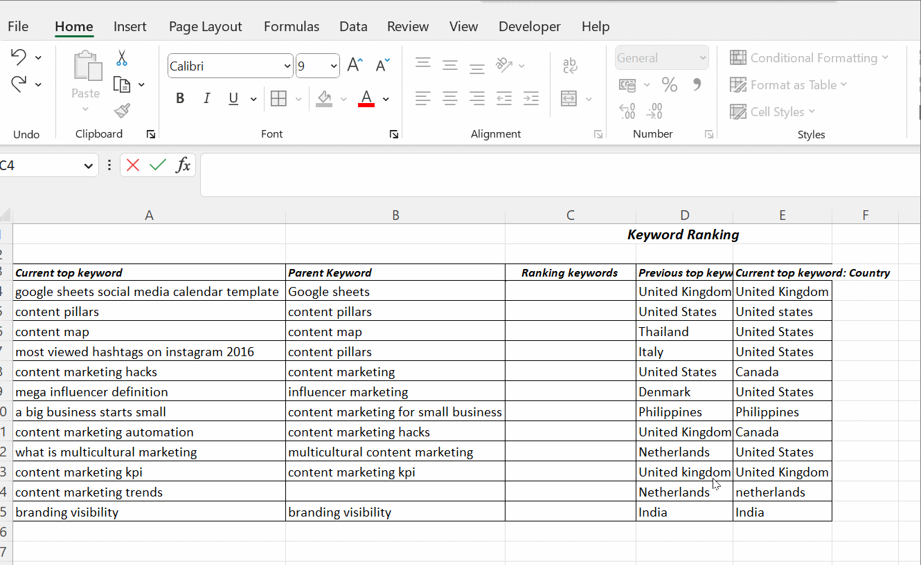
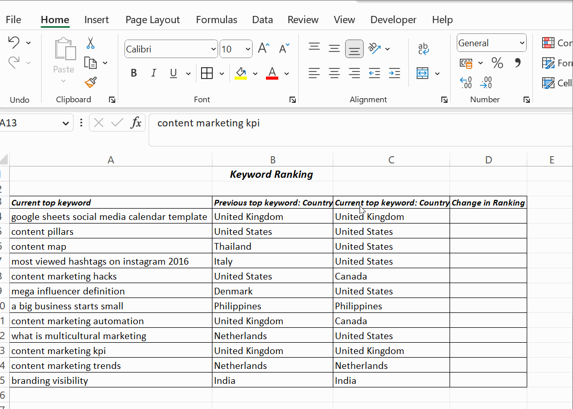
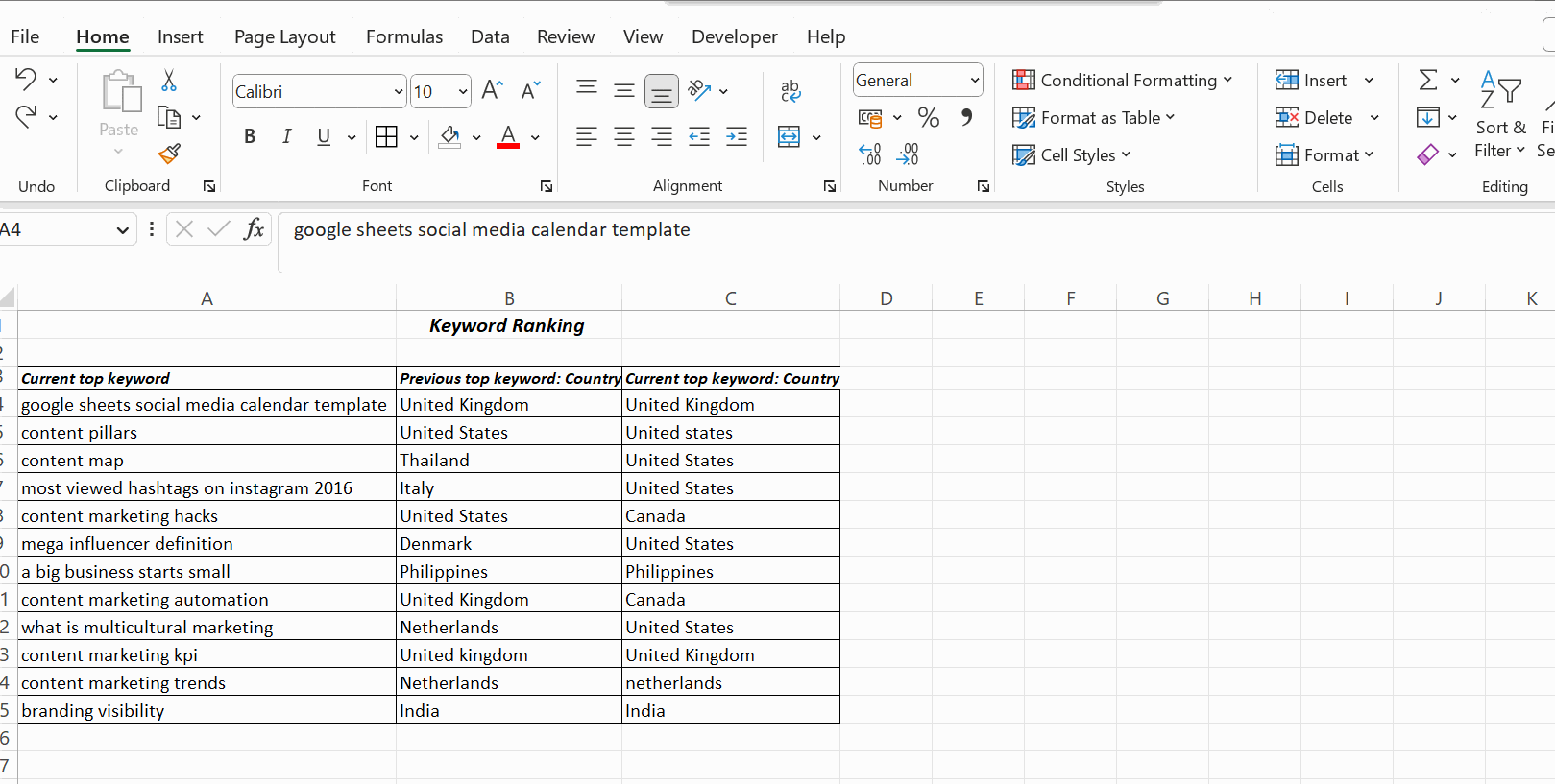
Column A contains a list of top keywords in a blog, and column B is the parent keyword. The resulting comparison must return all the ranking keywords in the blog.
The VLOOKUP() is applied in cell C4 as =VLOOKUP(A4, $B$4:$B$15,1,0).
Drag the cell to apply the formula in all the cells below C4. You will find the result in column C with the current and the matching parent keywords. The formula in Excel to compare two columns using VLOOKUP is as follows.
VLOOKUP(A4,..,..,..) - This takes the value in cell A4.
VLOOKUP(A4, $B$4:$B$15,..,..) - This compares all the values in cells from B4 to B15. That’s why the cells in range B4:B15 are locked using absolute reference. The $ symbol before the cell reference is called an absolute reference.
VLOOKUP(A4, $B$4:$B$15,1,..) - The third argument is the col_index_num, which mentions the position of the column to compare from the lookup value A4.
In the above example, the current top keyword is in column A, and the column with which it has to be compared is 1 column away. Hence, the value 1.
VLOOKUP(A4, $B$4:$B$15,1,0) - The last argument takes a logical value, either 0 or 1.
If you wish to find the exact match, mention 0(zero). If you want VLOOKUP() to return a closet match sorted in ascending order, mention 1 in this argument.
Frequently Asked Questions
1. How do you compare two columns in Excel?
When comparing two columns in Excel, one method is to select both columns of data, select Home → Find & Select → Go To Special → Row Differences, and click OK. The matching data cells across the columns' rows are white, and unmatched cells appear in gray.

2. How to compare three or more columns in Excel?
To find matches in all cells when the table has three or more columns, use an IF() with AND statement. The formula is =IF(AND(A2=B2, A2=C2), "Full match", "").
The formula to find matches in any two cells in the same row is =IF(OR(A2=B2, B2=C2, A2=C2), "Match", "").
Conclusion
It’s easy to compare two columns when the table in the spreadsheet is small. However, when the spreadsheets are vast or multiple spreadsheets are linked, the comparison starts to get complicated.
This tutorial briefed you on how to compare two columns in Excel. Microsoft Excel offers options to compare and match data in a single column, multiple columns, and multiple spreadsheets.
And if you want to excel in Microsoft Excel, check out our article, “The Top 5 Excel Functions to Make Work Easier,” to learn more about Excel functions and formulas. You can also explore Pitman Training’s Microsoft Excel Courses and Certificate to jumpstart your career and be ahead of the competition. Make sure to visit our website and expand your knowledge of Microsoft Office and Microsoft Word.